Problem Background
The purpose of this assignment is to familiarize oneself with numerical integration. One must evaluate a set of integrals using discrete sums of sufficient resolution to deliver a function which describes light waves near a cliff which has a size on the order of magnitude of the waves themselves.
Conveniently, the assignment describes both the problem and solution. Fresnel diffraction theory comes to the conclusion that light waves traveling perpendicular to an opaque barrier have an intensity $I$ as a function of $x_0$, the parallel distance from the edge of the barrier, which sits at $z$ above the observation plane:
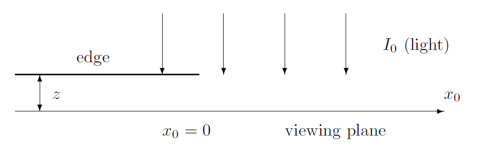
$$I\left(x_0\right) =\text { const. } \times\left|\int_0^{+\infty} \exp \left[\frac{i \pi}{\lambda z}\left(x_0-x\right)^2\right] d x\right|^2 =\frac{I_0}{\lambda z}\left|\int_{-\infty}^{x_0} \exp \left(\frac{i \pi x^2}{\lambda z}\right) d x\right|^2$$
Since this integral does not behave very well, the assignment suggests evaluating the following integrals instead, which break the same problem into equations which are easier to evaluate:
$$I(u_0) = \frac{1}{2}I_0\{[C(u_0)-C(-\infty)]^2+[S(u_0)-S(-\infty)]^2\}$$
$$C(u_0) = \int_{0}^{u_0}cos\left(\frac{\pi}{2}u^2\right)du$$
$$S(u_0) = \int_{0}^{u_0}sin\left(\frac{\pi}{2}u^2\right)du$$
$$u_0 = x_0\sqrt{\frac{2}{\lambda z}}$$
The value $u_0$ is a dimensionless parameter, and $C(-\infty) = S(-\infty) = 0.5$.
# The usual imports
import matplotlib.pyplot as plt
import numpy as np, scipy as sp
import math
plt.style.use('dark_background') #Don't judge me
plt.rcParams['figure.figsize'] = [20, 10]
Solution Description
Step one is to separate my trapezoid-rule-based integration method into a more generic function which can take any set of variables and functions to evaluate (provided that the integral is finite). I decided to set up this function to take either a number of points to use to evaluate the integral, or a tolerance value to achieve. If given a number of points, the numerical integration is performed in a straightforward way. If using a tolerance value, the integral is taken with a successively doubled number of intervals until the precision of the result stops changing by more than the tolerance value.
def trap_rule(xmin, xmax, func_eval, points = 0, tol = 0):
    if(points==0 and tol==0):
        raise Exception("Please define either a number of points, or a tolerance, with which an integral can be taken.")
    elif(points<0 or tol<0):
        raise Exception("Please define a positive tolerance or number of points.")
    elif(points>0 and tol>0):
        raise Exception("Please choose to either a number of points or a tolerance value.")
    #uses recursive form of the trapezoid rule to evaluate
    #func_eval between xmin and xmax to a tolerance of tol or
    #for a set of intervals=points-1
    if(points>0 and tol==0):
        if(points==1):
            raise Exception("Please choose at least 2 points of evaluation.")
        #calculate the integral based on intervals = points-1
        #print("Integral based on "+str(points-1)+" interval(s).")
        dx=(xmax-xmin)/(points-1)
        trap = 0.0
        i=1
        while(i<points-1): #add all trapezoids except first and last one
            trap = trap + func_eval(xmin+i*dx)
            i = i+1
        #add the first and last points as counted once (take average)
        result = (trap+0.5*(func_eval(xmin)+func_eval(xmax)))*dx
        return result #,points-1
    elif(points==0 and tol>0):
        #calculate the integral recursively based on tolerance
        #print("Integral to a tolerance of "+str(tol)+" units.")
        dx = (xmax-xmin) #width
        intervals = 1
        #starting approx is a single big trapezoid
        trap = 0.5*(func_eval(xmin)+func_eval(xmax)) #height
        integral_new = dx*trap #width*height
        integral_old = integral_new+2*tol #starting val
        #until we are precise,
        #keep doubling intervals and recalculating
        while abs(integral_new-integral_old)>abs(tol) or intervals<8:
            intervals = intervals*2
            dx = (xmax-xmin)/intervals
            integral_old = integral_new
            i=1
            while(i<intervals): #add in the in-between trapezoids
                trap = trap + func_eval(xmin+i*dx)
                i = i+2
            integral_new = (trap)*dx
        return integral_new#,intervals
Next I define variables and a couple of helper functions. In this case I find it easy to separate the integrand to the Fresnel integrals, since I'll be evaluating them repeatedly. Finally, a function is defined which computes the intensity function we are looking for.
#integrand of the Fresnel integrals, as lambda functions
fres_cos = lambda u: math.cos(math.pi*0.5*u*u)
fres_sin = lambda u: math.sin(math.pi*0.5*u*u)
#u_0 as a function of z, lambda, and x_0
u_0 = lambda x_0, l, z: x_0*((2/(l*z))**0.5)
#the Fresnel integrals themselves as a nexted lambda call
fres_C = lambda u_0, points=0, tol=0: trap_rule(0,u_0,fres_cos,points,tol)
fres_S = lambda u_0, points=0, tol=0: trap_rule(0,u_0,fres_sin,points,tol)
#constants and variables
C_inf = S_inf = -0.5
#finally we can use the above to define the intensity of the light as a function of u_0
def intensity(u_0, points=0, tol=0):
    #this computes I/I_0 where I_0 is the intensity of the light incident on the cliff's edge
    C_part = (fres_C(u_0, points, tol)-C_inf)
    S_part = (fres_S(u_0, points, tol)-S_inf)
    return 0.5*(C_part*C_part+S_part*S_part)
To show the precision increase as a function of evaluation points, I first chart the intensity result when $u_0 = 0.5$ and for $u_0 = 3$ for $n = 4, 8, 16, ..., 8192$ points during integral evaluation.
u_is_3 = np.empty(12)
u_is_p5 = np.empty(12)
i=0
for n in range(2,14):
    u_is_3[i] = intensity(3,points = 2**n)
    u_is_p5[i] = intensity(0.5,points = 2**n)
    i = i+1
print("\t\tu_0 = 0.5 \t\tu_0 = 3")
for i in range(len(u_is_p5)):
    print("points: "+str(2**(i+2)), end="\t")
    print(u_is_p5[i],end = "\t")
    print(u_is_3[i])
		u_0 = 0.5 		u_0 = 3
points: 4	0.6523764475540318	3.9999999999999996
points: 8	0.6519305710316761	0.9226875214725248
points: 16	0.6518555837174023	1.0714732514522431
points: 32	0.6518397290998141	1.0994203097242432
points: 64	0.6518360625363202	1.105655393288219
points: 128	0.6518351797726517	1.1071441762281402
points: 256	0.6518349631320459	1.1075088134568198
points: 512	0.651834909467208	1.107599094860617
points: 1024	0.6518348961122434	1.107621559451759
points: 2048	0.651834892781117	1.1076271626222505
points: 4096	0.6518348919492836	1.1076285618076962
points: 8192	0.6518348917414453	1.107628911404094
In order to achieve 4 or 5 digits of precision, I need about 256 points in the case where $u_0 = 0.5$, and closer to 512 points in the case where $u_0 = 3$. Luckily, I've defined my trapezoid rule function such that I can input a tolerance value instead of a number of points. Therefore I will simply enter $tol = .00001$ to achieve the precision that I need. Using the intensity as a function of $u_0$ I can now define intensity_in_space which computes my final graph of light intensity along the viewing plate.
def intensity_in_space(xmin, xmax, wavlen, zdist, num, points = 0, tol = 0):
    data = [0]*num
    xaxis = [0]*num
    delta = (xmax-xmin)/(num-1)
    for i in range(num-1):
        xaxis[i] = xmin+i*delta
        data[i] = intensity(u_0(xaxis[i],wavlen,zdist),points,tol)
    xaxis[num-1] = xmax
    data[num-1] = intensity(u_0(xmax,wavlen,zdist),points,tol)
    return xaxis, data
Plotting a few hundred points from -1 micron to 4 microns, I can confirm the validity of the solution with a few limit checks.
data = intensity_in_space(-1e-6, 4e-6, 0.5e-6, 1e-6, 500, tol=.00001)
plt.plot(data[0],data[1])
plt.title("Relative Intensity as a Function of Distance",fontsize = "20")
plt.xlabel(r"distance from ledge (m)",fontsize = "20");
plt.ylabel(r"$\frac{I}{I_0}$",fontsize = "20");

The first thing to check is that $I/I_0$ at $x_0 = 0$ is 0.25, one of the only analytically calculable points. The next thing is that we approach zero to the left which is further from the opening. This makes sense if the opaque barrier extends to negative infinity. The last is the fact that as $x_0$ gets very large, both of the Fresnel integrals approach 0.5.
$$C(\infty) = \int_{0}^{\infty}cos\left(\frac{\pi}{2}u^2\right)du = 0.5$$
$$S(\infty) = \int_{0}^{\infty}sin\left(\frac{\pi}{2}u^2\right)du = 0.5$$
$$I(u_0) = \frac{1}{2}I_0\{[C(\infty)-C(-\infty)]^2+[S(\infty)-S(-\infty)]^2\} = \frac{1}{2}I_0\{[0.5-(-0.5)]^2+[0.5-(-0.5)]^2\} = I_0$$
Therefore, the realtive intensity should approach 1, which the graph shows accurately.